A Simple Proof for the Gap Between the Muon and RMNP Descent Directions on Linear Regression
1. Setup
Here I only discuss the simplest possible example. The corresponding statement for neural networks is much more intricate and requires substantially deeper analysis. Consider the basic linear-regression loss
\[L(W) = \tfrac{1}{2}\|W\|_F^2\]whose gradient is $\nabla L = W$. Under this loss, the descent directions of Muon and RMNP are
- Muon: $(WW^T)^{-1/2}\,W$
- RMNP: $\mathrm{diag}(WW^T)^{-1/2}\,W$
The core question is: under random initialization, how large can the gap between these two directions be? Equivalently, we study norms of
\[\Delta := (WW^T)^{-1/2}W - \mathrm{diag}(WW^T)^{-1/2}W.\]Notation.
- $A := WW^T$
- $D := \mathrm{diag}(WW^T)$, with $D_{ii} = |W_{i\ast}|^2$
- $E := A - D$, with $E_{i\ell} = \langle W_{i\ast}, W_{\ell\ast}\rangle$ for $i \neq \ell$
2. Main Theorem
Main theorem. Let $W \in \mathbb{R}^{m \times n}$ with $W_{ij} \stackrel{\text{iid}}{\sim} \mathcal{N}(0,1)$, and keep $m$ fixed. Then there exist positive constants $c_1, c_2, C$, depending only on $m$, such that whenever $n \geq C$:
(A) High-probability operator-norm bound
\[\mathbb{P}\bigl[\|\Delta\|_{\mathrm{op}} \leq c_1/\sqrt n\bigr] \geq 1 - n^{-2}\](B) High-probability Frobenius-norm bound
\[\mathbb{P}\bigl[\|\Delta\|_F \leq c_2/\sqrt n\bigr] \geq 1 - n^{-2}\]3. Lemmas
3.1 Balakrishnan integral representation
For any positive definite matrix $X \succ 0$,
\[X^{-1/2} = \frac{1}{\pi}\int_0^\infty t^{-1/2}(X+tI)^{-1}\,dt.\]Proof. After spectral decomposition, it reduces to the scalar identity
\[\lambda^{-1/2} = \frac{1}{\pi}\int_0^\infty\frac{dt}{\sqrt t(\lambda+t)}.\]Substitute $t = \lambda u$ to obtain
\[\frac{1}{\sqrt\lambda}\cdot\frac{1}{\pi}\int_0^\infty\frac{du}{\sqrt u(1+u)} = \frac{1}{\sqrt\lambda},\]and use $B(1/2,1/2) = \pi$. $\square$
Reference: Higham, Functions of Matrices (2008).
3.2 A scalar integral
For $a, b > 0$,
\[\int_0^\infty \frac{dt}{\sqrt t\,(a+t)(b+t)} = \frac{\pi}{\sqrt{ab}(\sqrt a+\sqrt b)}.\]Proof. Substitute $t = s^2$, so $dt = 2s\,ds$:
\[2\int_0^\infty\frac{ds}{(a+s^2)(b+s^2)} = \frac{2}{b-a}\int_0^\infty\left[\frac{1}{a+s^2}-\frac{1}{b+s^2}\right]ds = \frac{\pi}{\sqrt{ab}(\sqrt a+\sqrt b)}.\]$\square$
3.3 Davidson-Szarek inequality
Let $W \in \mathbb{R}^{m\times n}$ with $m \leq n$ and $W_{ij}\stackrel{\text{iid}}{\sim}\mathcal{N}(0,1)$. For every $t > 0$,
\[\mathbb{P}\bigl[\sigma_{\max}(W) \geq \sqrt n + \sqrt m + t\bigr] \leq e^{-t^2/2}\]and
\[\mathbb{P}\bigl[\sigma_{\min}(W) \leq \sqrt n - \sqrt m - t\bigr] \leq e^{-t^2/2}.\]Reference: Vershynin, High-Dimensional Probability (2018).
3.4 Laurent-Massart concentration for $\chi^2$
Let $Z \sim \chi^2_n$. For every $x > 0$,
\[\mathbb{P}\bigl[Z \geq n + 2\sqrt{nx} + 2x\bigr] \leq e^{-x},\qquad \mathbb{P}\bigl[Z \leq n - 2\sqrt{nx}\bigr] \leq e^{-x}.\]Reference: B. Laurent and P. Massart (2000), Ann. Stat. 28(5), 1302-1338.
3.5 A high-probability event
Define
\[\Omega_n := \{\sigma_{\min}(W)\geq\sqrt n/2\}\cap\{\sigma_{\max}(W)\leq 2\sqrt n\}\cap\{\min_i D_{ii}\geq n/2\}\cap\{\|E\|_{\mathrm{op}}\leq c_0\sqrt n\},\]where $c_0$ depends only on $m$. Then for sufficiently large $n$,
\[\mathbb{P}(\Omega_n^c) \leq n^{-2}.\]Proof.
(a) Bounds on singular values. Apply Davidson-Szarek from Section 3.3 with $t = \sqrt n/4$. When $n \geq 16m$,
\[\mathbb{P}\bigl[\sigma_{\max}(W) \leq 2\sqrt n\bigr] \geq 1 - e^{-n/32},\qquad \mathbb{P}\bigl[\sigma_{\min}(W) \geq \tfrac{\sqrt n}{2}\bigr] \geq 1 - e^{-n/32}.\](b) Bounds on row norms. Since $D_{ii} = |W_{i\ast}|^2\sim\chi^2_n$, applying Laurent-Massart from Section 3.4 with $x = n/16$ gives
\[\mathbb{P}[D_{ii} \leq n/2] \leq e^{-n/16}.\]Taking a union bound over $i = 1, \ldots, m$ yields
\[\mathbb{P}\bigl[\min_i D_{ii} \geq n/2\bigr] \geq 1 - m e^{-n/16}.\](c) A bound on $|E|_{\mathrm{op}}$. Each off-diagonal entry
\[E_{i\ell} = \sum_{k=1}^n W_{ik}W_{\ell k}, \qquad i \neq \ell,\]is a sum of $n$ independent mean-zero sub-exponential random variables. Bernstein’s inequality gives
\[\mathbb{P}[|E_{i\ell}|\geq u] \leq 2\exp\!\bigl(-c\min(u^2/n, u)\bigr).\]Choosing $u = c_0’\sqrt n$ with $c_0’$ large enough gives probability at least $1 - e^{-c’n}$. Taking a union bound over the $\binom{m}{2}$ pairs still leaves probability at least $1 - m^2 e^{-c’n}$.
Using the crude bound
\[\|E\|_{\mathrm{op}}\leq m\cdot\max_{i,\ell}|E_{i\ell}|\leq c_0\sqrt n\]with $c_0 = m c_0’$, we conclude the claim.
Finally, combining the three bad events in (a), (b), and (c), each of which has exponentially small probability, shows that for all sufficiently large $n$ their total probability is at most $n^{-2}$. $\square$
3.6 An exact perturbation identity
For positive definite $A, D \succ 0$,
\[A^{-1/2}-D^{-1/2} = -\frac{1}{\pi}\int_0^\infty t^{-1/2}(A+tI)^{-1}E(D+tI)^{-1}\,dt.\]Proof. Apply the Balakrishnan representation from Section 3.1 to both $A$ and $D$, subtract, and use the algebraic identity $X^{-1}-Y^{-1} = -X^{-1}(X-Y)Y^{-1}$ with $X=A+tI$, $Y=D+tI$, and $X-Y=E$. $\square$
3.7 A deterministic operator-norm bound
For all positive definite $A, D \succ 0$,
\[\|A^{-1/2}-D^{-1/2}\|_{\mathrm{op}} \leq \frac{\|E\|_{\mathrm{op}}}{ \sqrt{\lambda_{\min}(A)\,\lambda_{\min}(D)} \left(\sqrt{\lambda_{\min}(A)}+\sqrt{\lambda_{\min}(D)}\right) }.\]Proof. Take operator norms in the exact perturbation identity from Section 3.6, use $\lVert XYZ\rVert_{\mathrm{op}}\leq\lVert X\rVert_{\mathrm{op}}\lVert Y\rVert_{\mathrm{op}}\lVert Z\rVert_{\mathrm{op}}$, and then apply the scalar integral from Section 3.2. $\square$
4. Proof of the Main Theorem
4.1 Proof of (A): the operator-norm bound
On the event $\Omega_n$ from Section 3.5,
- $\lambda_{\min}(A) = \sigma_{\min}(W)^2 \geq n/4$
- $\lambda_{\min}(D) \geq n/2$
- $|E|_{\mathrm{op}}\leq c_0\sqrt n$
- $|W|_{\mathrm{op}}\leq 2\sqrt n$
Substituting into the deterministic bound from Section 3.7, the denominator satisfies
\[\sqrt{(n/4)(n/2)}\cdot(\sqrt{n/4}+\sqrt{n/2}) \geq c_4 n^{3/2},\]so
\[\|A^{-1/2}-D^{-1/2}\|_{\mathrm{op}}\leq \frac{c_0\sqrt n}{c_4 n^{3/2}} = \frac{c_5}{n}.\]Since $\Delta = (A^{-1/2}-D^{-1/2})W$, we get
\[\|\Delta\|_{\mathrm{op}}\leq \frac{c_5}{n}\cdot 2\sqrt n = \frac{c_1}{\sqrt n}.\]Because $\mathbb{P}(\Omega_n) \geq 1 - n^{-2}$ by Section 3.5, this proves part (A). $\square$
4.2 Proof of (B): the Frobenius-norm bound
The matrix $\Delta$ has size $m\times n$, with $m$ fixed. Hence
\[\|\Delta\|_F\leq\sqrt m\cdot\|\Delta\|_{\mathrm{op}}.\]Therefore, on $\Omega_n$,
\[\|\Delta\|_F\leq \sqrt m\cdot\frac{c_1}{\sqrt n} = \frac{c_2}{\sqrt n}.\]The same probability bound $1-n^{-2}$ then proves part (B). $\square$
5. Conclusion and Discussion
5.1 Summary
| Quantity | Estimate | Probability |
|---|---|---|
| $|\Delta|_{\mathrm{op}}$ | $\leq c_1/\sqrt n$ | $\geq 1 - n^{-2}$ |
| $|\Delta|_F$ | $\leq c_2/\sqrt n$ | $\geq 1 - n^{-2}$ |
All constants $c_i$ depend only on the fixed row dimension $m$, and not on $n$.
5.2 Intuition
Returning to the basic linear-regression loss $L(W) = \tfrac{1}{2}|W|_F^2$, when $n\to\infty$ with $m$ fixed, the Muon descent direction $(WW^T)^{-1/2}W$ and the RMNP descent direction $\mathrm{diag}(WW^T)^{-1/2}W$ become asymptotically identical in probability, with gap size $\Theta(1/\sqrt n)$.
The source of the gap is exactly the off-diagonal part $E$ of $WW^T$. The entry $E_{i\ell} = \langle W_{i\ast}, W_{\ell\ast}\rangle$ measures the correlation between row $i$ and row $\ell$. In high dimension, when $n\gg m$, independent random vectors are nearly orthogonal, so these off-diagonal terms are of relative order $O(1/\sqrt n)$.
The source of the gap is exactly the off-diagonal part $E$ of $WW^T$. The entry $E_{i\ell} = \langle W_{i\ast}, W_{\ell\ast}\rangle$ measures the correlation between row $i$ and row $\ell$. In high dimension, when $n\gg m$, independent random vectors are nearly orthogonal, so these off-diagonal terms are of relative order $O(1/\sqrt n)$.
Intuitively, RMNP normalizes each row independently and produces $m$ unit vectors. Muon then applies a small correction to make them exactly orthogonal. Once pairwise inner products are already of order $O(1/\sqrt n)$, that correction must itself also be of order $O(1/\sqrt n)$.
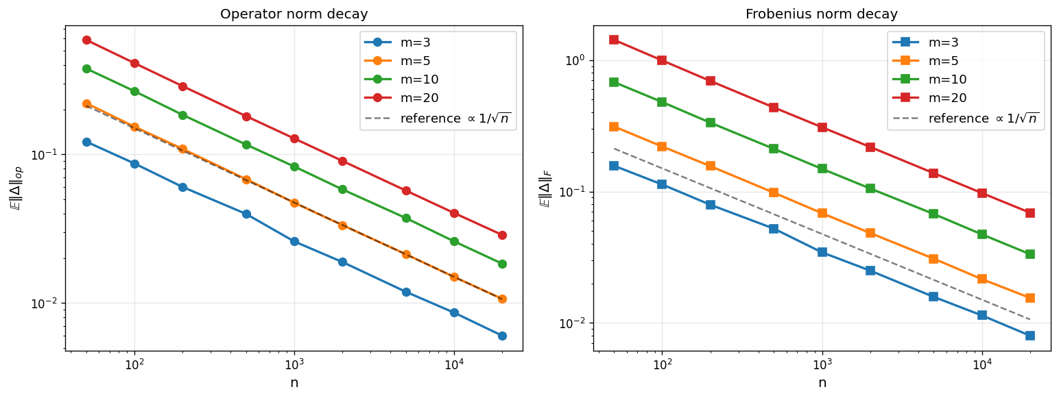
6. Numerical Experiment
6.1 Experimental setup
- Let $m \in {3, 5, 10, 20}$, and run one experiment for each fixed value of $m$
- For each $m$, let $n$ range over ${50, 100, 200, 500, 1000, 2000, 5000, 10000, 20000}$
- Run 500 Monte Carlo samples for each $(m, n)$ pair
- Sample each $W_{ij}$ independently from $\mathcal{N}(0,1)$
- Compute $(WW^T)^{-1/2}$ by symmetric eigendecomposition: if $WW^T = U\Lambda U^T$, then $(WW^T)^{-1/2} = U\Lambda^{-1/2}U^T$
6.2 Results
$m = 3$:
| $n$ | $\mathbb{E}|\Delta|_{\mathrm{op}}$ | $\mathbb{E}|\Delta|_F$ |
|---|---|---|
| 50 | 0.122 | 0.157 |
| 100 | 0.087 | 0.113 |
| 200 | 0.060 | 0.079 |
| 500 | 0.040 | 0.052 |
| 1000 | 0.026 | 0.034 |
| 2000 | 0.019 | 0.025 |
| 5000 | 0.012 | 0.016 |
| 10000 | 0.009 | 0.011 |
| 20000 | 0.006 | 0.008 |
$m = 5$:
| $n$ | $\mathbb{E}|\Delta|_{\mathrm{op}}$ | $\mathbb{E}|\Delta|_F$ |
|---|---|---|
| 50 | 0.221 | 0.312 |
| 100 | 0.154 | 0.220 |
| 200 | 0.109 | 0.156 |
| 500 | 0.068 | 0.098 |
| 1000 | 0.047 | 0.068 |
| 2000 | 0.033 | 0.048 |
| 5000 | 0.021 | 0.031 |
| 10000 | 0.015 | 0.022 |
| 20000 | 0.011 | 0.015 |
$m = 10$:
| $n$ | $\mathbb{E}|\Delta|_{\mathrm{op}}$ | $\mathbb{E}|\Delta|_F$ |
|---|---|---|
| 50 | 0.378 | 0.680 |
| 100 | 0.266 | 0.480 |
| 200 | 0.185 | 0.334 |
| 500 | 0.116 | 0.211 |
| 1000 | 0.083 | 0.149 |
| 2000 | 0.058 | 0.105 |
| 5000 | 0.037 | 0.067 |
| 10000 | 0.026 | 0.047 |
| 20000 | 0.018 | 0.033 |
$m = 20$:
| $n$ | $\mathbb{E}|\Delta|_{\mathrm{op}}$ | $\mathbb{E}|\Delta|_F$ |
|---|---|---|
| 50 | 0.589 | 1.426 |
| 100 | 0.412 | 0.994 |
| 200 | 0.288 | 0.694 |
| 500 | 0.181 | 0.436 |
| 1000 | 0.128 | 0.308 |
| 2000 | 0.090 | 0.218 |
| 5000 | 0.057 | 0.138 |
| 10000 | 0.040 | 0.097 |
| 20000 | 0.029 | 0.069 |
6.3 Conclusion
For each fixed $m$, both norms are parallel to the reference line $1/\sqrt n$ in log-log coordinates, verifying
\[\mathbb{E}\|\Delta\|_{\mathrm{op}} = \Theta(1/\sqrt n),\qquad \mathbb{E}\|\Delta\|_F = \Theta(1/\sqrt n).\]The curves for different values of $m$ are themselves parallel to one another, with the same slope $-1/2$ and only different constant factors. This further confirms that the asymptotic regime of “fixed $m$, $n\to\infty$” is independent of the particular value of $m$.
The experimental results match the theoretical prediction exactly.