Row Normalization and Orthogonalization Are Asymptotically Equivalent on Neural Networks
TL;DR. On neural networks, two seemingly different matrix-level preconditioners turn out to be asymptotically equivalent: orthogonalization, and row-wise $\ell_2$ normalization along the input dimension. We provide preliminary theoretical results for this picture together with large-scale empirical evidence. On the theoretical side, we give a closed-form analysis of the gradient self outer-product across three canonical NN-theory setups at initialization (matrix factorization, deep linear networks, and 2-layer ReLU networks), and our results show that row normalization and orthogonalization are asymptotically equivalent in these setups. On the empirical side, we track the full training dynamics of GPT-2 and LLaMA at multiple scales, and verify that orthogonalization and row-wise normalization remain approximately equivalent throughout training. Taken together, these two analyses clarify a long-standing puzzle: why does orthogonalization-based preconditioning adapt so well to the curvature structure of neural networks? The answer is that its action is implicitly aligned with the block-diagonally-dominant Hessian of neural networks.
1. Muon
Muon [1] optimizes matrix-shaped weights $W_t \in \mathbb{R}^{m \times n}$ with a momentum-based update. Given a stochastic gradient $G_t = \nabla f(W_t; \xi^t)$ at step $t$, its full algorithm is
\[\begin{aligned} G_t &= \nabla f(W_t; \xi^t), \\ V_t &= \beta V_{t-1} + (1 - \beta) G_t, \\ D_t &= \mathrm{NS}_5(V_t) \approx (V_t V_t^\top)^{-1/2} V_t, \\ W_{t+1} &= W_t - \eta_t D_t, \end{aligned}\]with $V_0 = 0$, momentum coefficient $\beta \in [0, 1)$, and learning rate $\eta_t > 0$. The defining feature is the descent direction $D_t$: rather than using the momentum $V_t$ directly, Muon orthogonalizes it. If we apply the SVD to do the orthogonalization, we will have:
\[D_t \;=\; U V^\top \;=\; (V_t V_t^\top)^{-1/2}\, V_t,\]2. How Muon Adapts to the Hessian Structure of Neural Networks
As a preconditioned optimizer, how does Muon adapt to the Hessian structure of neural networks? This is a fundamental question. Simple preconditioned methods like Muon were only very recently found to dramatically outperform other optimizers on neural networks, and no analysis under the classical optimization theory setup predicts such a gap. The shortfall is no accident — classical theory studies worst-case problems within an abstract problem class (typically steepest descent on nonconvex smooth problem classes), and worst-case analyses are by construction blind to the structural properties of the actual problems they are applied to. To explain Muon’s effectiveness, we have to look at the structure of neural networks themselves.
A line of empirical and theoretical work [2,3,4] has established that the layer-wise Hessian of a neural network is row-block diagonally dominant: when the Hessian of a weight matrix $W \in \mathbb{R}^{m \times n}$ is unfolded along the $m$ row-direction blocks of size $n \times n$, the diagonal blocks dominate the off-diagonal ones in magnitude.
Since the Hessian is the optimal preconditioner under a quadratic approximation of the loss, this row-block structure tells us what shape a good preconditioner should have.
If the implicit Muon preconditioner $H$ on the parameter is written via a Kronecker product, one can find that
\[H_{\mathrm{MUON}} \;=\; P_t^{1/2} \otimes I_n, \qquad P_t \;:=\; V_t V_t^\top.\]The structure of Muon’s preconditioner is therefore entirely determined by the structure of $V_t V_t^\top$. Comparing to the Hessian picture: if $V_t V_t^\top$ is diagonal, then $H_{\mathrm{MUON}} = P_t^{1/2} \otimes I_n$ is block-diagonal in exactly the row-block structure that the Hessian itself takes.
This raises a clean structural question:
Is $V_t V_t^\top$ (equivalently, $G_t G_t^\top$) diagonally dominant for neural networks?
For neural-network weight matrices, the answer is yes in the asymptotic-width regime.
This blog gives preliminary theoretical results on three canonical NN-theory setups (matrix factorization, deep linear networks, and 2-layer ReLU networks) at initialization that point to this conclusion; full-dynamics empirical evidence on practical models (GPT-2, LLaMA) is given in our paper [5]. Figure 2 summarizes this structural comparison: Muon’s preconditioner is row-block aligned precisely when $V_t V_t^\top$ is close to diagonal, matching the dominant row-block pattern observed in the neural-network Hessian.
3. Theoretical Understanding on NN Setup
If you do not want to go through the detailed theory, feel free to jump directly to Section 4 for the empirical evidence in practical training.
This blog gives an asymptotic analysis of the gradient self outer-product at initialization across three canonical NN-theory setups. Since the math gets fairly involved in each case, this blog only states the result for the 2-layer ReLU case and uses it to convey the picture; the full proofs are in the corresponding proof notes.
| Model | Setup | Proof note |
|---|---|---|
| Matrix factorization | \(\mathcal{L}(U) := \tfrac{1}{4} \| U U^\top - M^\star \|_F^2,\ U \in \mathbb{R}^{d \times k}\) | note |
| Deep linear network | \(\mathcal{L}(W_1, \ldots, W_L) := \tfrac{1}{2} \mathbb{E}_x \| W_L \cdots W_1 x - \Phi x \|^2\) | note |
| 2-layer ReLU | \(\mathcal{L}(W_1, W_2) := \tfrac{1}{2} \mathbb{E}_x \| W_2 \sigma(W_1 x) - \Phi x \|^2\) | note |
3.1 Setup
Let $d_0$ be the input dimension, $d_1$ the hidden dimension (this is the asymptotic axis of interest), and $d_2$ the output dimension. The two-layer ReLU network
\[f(x) \;=\; W_2\, \sigma(W_1 x), \qquad W_1 \in \mathbb{R}^{d_1 \times d_0}, \quad W_2 \in \mathbb{R}^{d_2 \times d_1},\]acts on inputs $x \in \mathbb{R}^{d_0}$ via $\sigma(z) := \max(z, 0)$. Write $h(x) := \sigma(W_1 x) \in \mathbb{R}^{d_1}$ and $w_a \in \mathbb{R}^{d_0}$ for the $a$-th row of $W_1$. The population loss against a deterministic linear target $\Phi \in \mathbb{R}^{d_2 \times d_0}$ is
\[\mathcal{L}(W_1, W_2) \;:=\; \tfrac{1}{2}\, \mathbb{E}_x \| W_2\, \sigma(W_1 x) - \Phi x \|^2,\]and let $G_{i,t} := \partial \mathcal{L} / \partial W_i$. At step $t = 0$ the momentum equals the gradient, $V_0 = G_0$, so $V_t V_t^\top = G_t G_t^\top$.
Standing assumption. At initialization,
\[(W_1)_{ij}, (W_2)_{ij} \stackrel{\mathrm{iid}}{\sim} \mathcal{N}(0, 1), \qquad x \sim \mathcal{N}(0, I_{d_0}),\]and $\Phi$ is deterministic and independent of $W_1, W_2$.
3.2 Closed-Form Structure of the Gradient Self Outer-Product
Theorem 1 (Structure of $\mathbb{E}[G_{2,t} G_{2,t}^\top]$).
\[\mathbb{E}[G_{2,t} G_{2,t}^\top] \;=\; \alpha\, I_{d_2} \;+\; \frac{d_1}{4}\, \Phi \Phi^\top,\]where $\alpha := \mathbb{E}_{W_1}[\mathrm{tr}(H^2)]$ with $H := \mathbb{E}_x[h(x) h(x)^\top]$, and $\alpha = \Theta(d_0^2 d_1^2)$ as $d_0, d_1 \to \infty$.
Theorem 2 (Structure of $\mathbb{E}[G_{1,t} G_{1,t}^\top]$). $\mathbb{E}[G_{1,t} G_{1,t}^\top]$ is permutation-invariant in the hidden index. Its diagonal entries are
\[\mathbb{E}[(G_{1,t} G_{1,t}^\top)_{aa}] \;=\; \frac{d_0 d_2^2}{4} \;+\; d_0 d_2\!\left[(d_1 - 1)\kappa_1 + \tfrac{1}{2}\right] \;+\; \frac{\|\Phi\|_F^2}{4},\]and for $a \neq c$,
\[\mathbb{E}[(G_{1,t} G_{1,t}^\top)_{ac}] \;=\; d_0 d_2\, \kappa_2 \;+\; O(d_2 \sqrt{d_0}),\]where $\kappa_1, \kappa_2$ are dimension-free constants involving the angle between two i.i.d. standard Gaussians (as $d_0 \to \infty$, $\kappa_1 \to 1/(4\pi^2) + 1/16$ and $\kappa_2 \to 1/(4\pi)$).
3.3 Diagonal Dominance Follows Asymptotically
Summary of the leading orders from Theorems 1 and 2:
| Diagonal entries | Off-diagonal entries | |
|---|---|---|
| \(\mathbb{E}[G_{2,t} G_{2,t}^\top]\) | \(\Theta(d_0^2 d_1^2) + \tfrac{d_1}{4}(\Phi \Phi^\top)_{aa}\) | \(\tfrac{d_1}{4}(\Phi \Phi^\top)_{ac}\) |
| \(\mathbb{E}[G_{1,t} G_{1,t}^\top]\) | \(\Theta(d_0 d_2^2 + d_0 d_1 d_2)\) | \(\Theta(d_0 d_2)\) |
The asymptotic regime of interest is $d_1 \to \infty$ with the input dimension $d_0$ and output dimension $d_2$ held fixed — this is the hidden-width limit. Reading the table along the $d_1$ axis: the diagonal of $\mathbb{E}[G_{1,t} G_{1,t}^\top]$ scales as $\Theta(d_1)$ while the off-diagonal stays $\Theta(1)$. The diagonal-dominance ratio is therefore
\[\frac{\mathbb{E}[(G_{1,t} G_{1,t}^\top)_{aa}]}{\mathbb{E}[(G_{1,t} G_{1,t}^\top)_{ac}]} \;=\; \Theta(d_1).\]In particular, as the hidden width $d_1 \to \infty$, $G_{1,t} G_{1,t}^\top$ is asymptotically diagonal: the diagonal entries dominate the off-diagonal entries by a factor that grows linearly in the hidden width.
This mechanism is not hard to understand. In high dimensions, independent Gaussian vectors are orthogonal in expectation, which matches the behavior of the off-diagonal terms; meanwhile, the expected self-inner-product of a Gaussian vector grows with dimension, which matches the diagonal terms. Here the hidden width plays the role of that dimension: the strong independence across rows at initialization induces a similar near-orthogonality structure across gradient rows. As the hidden width grows, the off-diagonal terms grow more slowly than the diagonal ones, so $G_{1,t} G_{1,t}^\top$ becomes asymptotically diagonally dominant.
This 0-step result is the simplest model in which the dominance phenomenon is analytically transparent. The next section shows that the same structural force acts throughout training in practice.
4. Empirical Evidence Across Full Training Dynamics
To test whether this phenomenon persists in realistic models, our paper [5] experimentally studied the full training dynamics of GPT-2 and LLaMA. We found that $V_t V_t^\top$ remains diagonally dominant beyond the toy setting, and that this structure continues to appear throughout training. Concretely, for every matrix parameter, we tracked the row-wise dominance ratio
\[r_i \;:=\; \frac{(V_t V_t^\top)_{ii}}{\frac{1}{m-1}\sum_{j \neq i} |(V_t V_t^\top)_{ij}|},\]and aggregated it into per-layer minima, averages, and maxima ($r_{\min}, r_{\mathrm{avg}}, r_{\max}$), then averaged those across all matrix parameters in the network ($\bar r_{\min}, \bar r_{\mathrm{avg}}, \bar r_{\max}$).
Three observations:
- The ratios cross $1$ early and stay above it. After warm-up, $\bar r_{\min}, \bar r_{\mathrm{avg}}, \bar r_{\max}$ all rise above $1$ within the first few percent of training and remain there.
- Dominance grows with model scale. For both architectures, $\bar r_{\mathrm{avg}}$ and $\bar r_{\min}$ are visibly higher for larger models, consistent with the $\Theta(d_1)$ asymptotic scaling predicted by Theorem 2.
- The phenomenon is architecture-agnostic. Both GPT-2 and LLaMA show the same qualitative behavior, suggesting the dominance is a generic property of well-conditioned Transformer training rather than an artifact of any specific design choice.
In short: across model families, model scales, and the entire course of training, $V_t V_t^\top$ is not only diagonally dominant, but this dominance also becomes stronger as model scale increases.
5. RMNP: An Efficient Surrogate for Muon
Now this blog can close the loop. Recall Muon’s update direction:
\[D_t^{\text{Muon}} \;=\; (V_t V_t^\top)^{-1/2}\, V_t.\]Suppose $V_t V_t^\top$ is diagonal. Then $V_t V_t^\top = \mathrm{diag}(V_t V_t^\top)$ trivially, and so
\[(V_t V_t^\top)^{-1/2} \;=\; \mathrm{diag}(V_t V_t^\top)^{-1/2}.\]The right-hand side acts row-by-row: if $V_{t,i:}$ denotes the $i$-th row of $V_t$, then $\mathrm{diag}(V_t V_t^\top){ii} = |V{t,i:}|_2^2$, and
\[\bigl[ \mathrm{diag}(V_t V_t^\top)^{-1/2}\, V_t \bigr]_{i,:} \;=\; \frac{V_{t,i:}}{\|V_{t,i:}\|_2}.\]That is, applying $(V_t V_t^\top)^{-1/2}$ when $V_t V_t^\top$ is diagonal is exactly $\ell_2$ normalization along the input dimension — each row of $V_t$ (a vector indexed by the input axis) is divided by its own $\ell_2$ norm. A similar operation was first considered from the perspective of norm-constrained steepest descent in [6].
Building on this observation, we propose RMNP (Row-Momentum Normalized Preconditioning), which replaces Muon’s orthogonalization step with this input-dimension normalization:
\[D_t^{\text{RMNP}} \;:=\; \mathrm{diag}(V_t V_t^\top)^{-1/2}\, V_t.\]Equivalently, the implicit RMNP preconditioner has the same Kronecker form as Muon’s but retains only the diagonal blocks of $P_t = V_t V_t^\top$:
\[H_{\mathrm{RMNP}} \;=\; \mathrm{diag}(P_t)^{1/2} \otimes I_n.\]
Combined with the diagonal-dominance results of the previous two sections, this gives a clean picture: as the model width grows to infinity, RMNP and Muon are asymptotically equivalent — the costly $\Theta(mn \min(m, n))$ orthogonalization step in Muon collapses to a simple $\Theta(mn)$ input-dimension $\ell_2$ normalization, with no loss of preconditioning quality on neural networks.
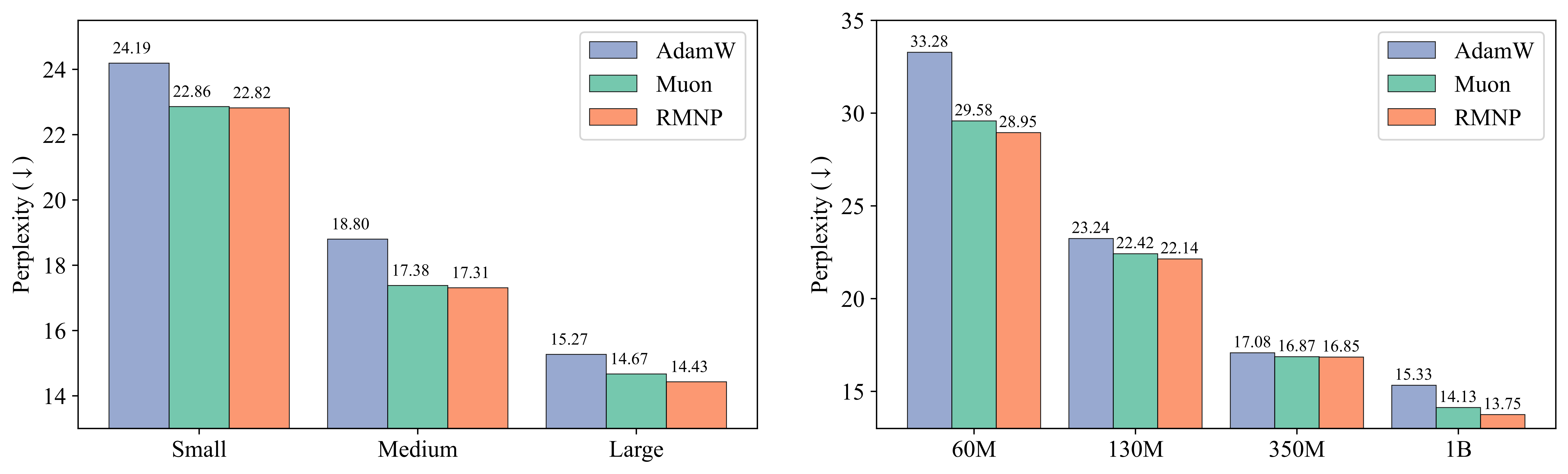
Our paper [5] shows that after multiple rounds of hyperparameter search for each optimizer RMNP provides comparable performance to Muon on GPT-2 (125M–1.5B) and LLaMA (60M–1B).
For further empirical results on row/column normalization and other advantages of normalization-based optimizers, please also see the following concurrent works:
- [7] A Minimalist Optimizer Design for LLM Pretraining.
- [8] SRON: State-Free LLM Training via Row-Wise Gradient Normalization.
- [9] Mano: Restriking Manifold Optimization for LLM Training.
- [10] On the Width Scaling of Neural Optimizers Under Matrix Operator Norms I: Row/Column Normalization and Hyperparameter Transfer.
- [13] Aurora: A Leverage-Aware Optimizer for Rectangular Matrices.
and earlier empirical explorations of various normalization schemes:
- [11] Gradient Multi-Normalization for Stateless and Scalable LLM Training.
- [12] SWAN: SGD with Normalization and Whitening Enables Stateless LLM Training.
- [6] Training Deep Learning Models with Norm-Constrained LMOs.
6. References
[1] Keller Jordan, Yuchen Jin, Vlado Boza, Jiacheng You, Franz Cesista, Laker Newhouse, and Jeremy Bernstein. Muon: An optimizer for hidden layers in neural networks. 2024. https://kellerjordan.github.io/posts/muon/
[2] Yushun Zhang, Congliang Chen, Tian Ding, Ziniu Li, Ruoyu Sun, and Zhi-Quan Luo. Why Transformers Need Adam: A Hessian Perspective. In Advances in Neural Information Processing Systems (NeurIPS), 2024. arXiv:2402.16788. https://arxiv.org/abs/2402.16788
[3] Yushun Zhang, Congliang Chen, Ziniu Li, Tian Ding, Chenwei Wu, Diederik P. Kingma, Yinyu Ye, Zhi-Quan Luo, and Ruoyu Sun. Adam-mini: Use Fewer Learning Rates To Gain More. arXiv preprint arXiv:2406.16793, 2024. https://arxiv.org/abs/2406.16793
[4] Zhaorui Dong, Yushun Zhang, Jianfeng Yao, and Ruoyu Sun. Towards Quantifying the Hessian Structure of Neural Networks. arXiv preprint arXiv:2505.02809, 2025. https://arxiv.org/abs/2505.02809
[5] Shenyang Deng, Zhuoli Ouyang, Tianyu Pang, Zihang Liu, Ruochen Jin, Shuhua Yu, and Yaoqing Yang. RMNP: Row-Momentum Normalized Preconditioning for Scalable Matrix-Based Optimization. In Proceedings of the 43rd International Conference on Machine Learning (ICML), 2026.
[6] Thomas Pethick, Wanyun Xie, Kimon Antonakopoulos, Zhenyu Zhu, Antonio Silveti-Falls, and Volkan Cevher. Training Deep Learning Models with Norm-Constrained LMOs. In Proceedings of the 42nd International Conference on Machine Learning (ICML), 2025. https://arxiv.org/abs/2502.07529
[7] Athanasios Glentis, Jiaxiang Li, Andi Han, and Mingyi Hong. A Minimalist Optimizer Design for LLM Pretraining. arXiv preprint arXiv:2506.16659, 2025. https://arxiv.org/abs/2506.16659
[8] Ziqing Wen, Yanqi Shi, Jiahuan Wang, Ping Luo, Linbo Qiao, Dongsheng Li, and Tao Sun. SRON: State-Free LLM Training via Row-Wise Gradient Normalization. OpenReview, 2025. https://openreview.net/forum?id=BtQLBWr6zI
[9] Yufei Gu and Zeke Xie. Mano: Restriking Manifold Optimization for LLM Training. arXiv preprint arXiv:2601.23000, 2026. https://arxiv.org/abs/2601.23000
[10] Ruihan Xu, Jiajin Li, and Yiping Lu. On the Width Scaling of Neural Optimizers Under Matrix Operator Norms I: Row/Column Normalization and Hyperparameter Transfer. arXiv preprint arXiv:2603.09952, 2026. https://arxiv.org/abs/2603.09952
[11] Meyer Scetbon, Chao Ma, Wenbo Gong, and Edward Meeds. Gradient Multi-Normalization for Stateless and Scalable LLM Training. arXiv preprint arXiv:2502.06742, 2025. https://arxiv.org/abs/2502.06742
[12] Chao Ma, Wenbo Gong, Meyer Scetbon, and Edward Meeds. SWAN: SGD with Normalization and Whitening Enables Stateless LLM Training. In Proceedings of the 42nd International Conference on Machine Learning (ICML), 2025. arXiv:2412.13148. https://arxiv.org/abs/2412.13148
[13] Alec Dewulf, Dhruv Pai, Li Yang, Ashley Zhang, and Ben Keigwin. Aurora: A Leverage-Aware Optimizer for Rectangular Matrices. Tilde Research Blog, 2026. https://blog.tilderesearch.com/blog/aurora
7. Citing This Blog
Cite. If you find this post useful, you may cite it as:
@misc{rmnp_blog_2026,
  title  = {Row Normalization and Orthogonalization Are Asymptotically Equivalent on Neural Networks},
  author = {Shenyang Deng},
  year   = {2026},
  note   = {Blog post},
  url    = {https://dsyforever.github.io/blog/normalization-orthogonalization/}
}
8. Acknowledgements
Thanks to Yushun Zhang, Shuhua Yu, and Yaoqing Yang for helpful discussions and feedback. Further acknowledgements may be added as this note evolves.